ISA Atmospheric Model
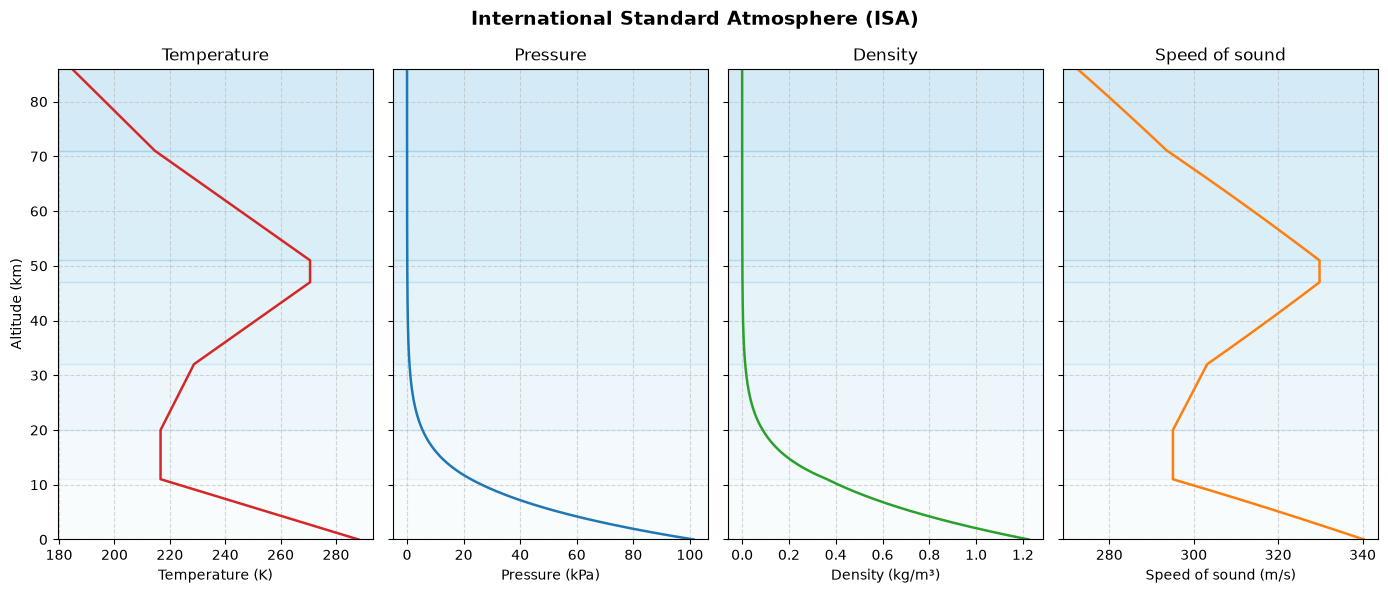
Compute temperature, pressure, density, and speed of sound from sea level to 86 km using the International Standard Atmosphere (ISA, ISO 2533:1975). Apply the model layer by layer, then plot each property against altitude.
[1]:
import numpy as np
import matplotlib.pyplot as plt
ISA Layer Definitions
Define each layer by its base geopotential altitude in meters, base temperature in kelvin, and temperature lapse rate in kelvin per meter.
[2]:
LAYERS = [
    # (base altitude m, base temperature K, lapse rate K/m)
    (0, 288.15, -0.0065),  # Troposphere
    (11_000, 216.65, 0.0),  # Tropopause (isothermal)
    (20_000, 216.65, +0.001),  # Lower stratosphere
    (32_000, 228.65, +0.0028),  # Upper stratosphere
    (47_000, 270.65, 0.0),  # Stratopause (isothermal)
    (51_000, 270.65, -0.0028),  # Lower mesosphere
    (71_000, 214.65, -0.002),  # Upper mesosphere
    (86_000, 186.87, 0.0),  # Mesopause boundary (limit)
]
[3]:
# Physical constants
R = 287.058  # Specific gas constant for dry air, J/(kg·K)
g0 = 9.80665  # Standard gravitational acceleration, m/s²
gamma = 1.4  # Ratio of specific heats for dry air
[4]:
# Sea-level reference values
T0 = 288.15  # K
P0 = 101_325  # Pa
rho0 = P0 / (R * T0)
Compute ISA Properties
Start with sea-level pressure. For each altitude, find the layer and compute the temperature from its base altitude and lapse rate:
The subscript b denotes the base of the current layer. In an isothermal layer, use the exponential pressure relation:
For a layer with a nonzero lapse rate, use:
Then compute density and speed of sound:
R is the specific gas constant for dry air, g0 is standard gravitational acceleration, and gamma is the ratio of specific heats.
[5]:
def isa_properties(altitudes_m: np.ndarray):
    """
    Compute ISA temperature, pressure, density, and speed of sound.

    Parameters
    ----------
    altitudes_m : numpy.ndarray
        Geopotential altitudes in meters.

    Returns
    -------
    T : numpy.ndarray
        Temperature in K.
    P : numpy.ndarray
        Pressure in Pa.
    rho : numpy.ndarray
        Air density in kg/m³.
    a : numpy.ndarray
        Speed of sound in m/s.

    """
    T = np.empty_like(altitudes_m)
    P = np.empty_like(altitudes_m)

    for i, h in enumerate(altitudes_m):
        # Find the layer containing altitude h.
        P_base = P0
        for layer_idx in range(len(LAYERS) - 1):
            h_base, T_b, L = LAYERS[layer_idx]
            h_top = LAYERS[layer_idx + 1][0]

            if h <= h_top:
                dh = h - h_base
                T[i] = T_b + L * dh
                if L == 0.0:
                    P[i] = P_base * np.exp(-g0 * dh / (R * T_b))
                else:
                    P[i] = P_base * (T[i] / T_b) ** (-g0 / (L * R))
                break
            else:
                # Compute pressure at the next layer boundary.
                dh = h_top - h_base
                T_top = T_b + L * dh
                if L == 0.0:
                    P_base = P_base * np.exp(-g0 * dh / (R * T_b))
                else:
                    P_base = P_base * (T_top / T_b) ** (-g0 / (L * R))

    rho = P / (R * T)
    a = np.sqrt(gamma * R * T)
    return T, P, rho, a
[6]:
# Altitude grid from sea level to 86 km
h = np.linspace(0, 86_000, 1_000)
[7]:
T, P, rho, a = isa_properties(h)
h_km = h / 1_000  # Convert to km for plotting.
Plot Atmospheric Properties
Plot each property against altitude. Shade the layers to show where the lapse rate changes.
[8]:
fig, axes = plt.subplots(1, 4, figsize=(14, 6), sharey=True)
fig.suptitle("International Standard Atmosphere (ISA)", fontsize=14, fontweight="bold")
# Shade the ISA layers.
layer_colors = [
    "#e8f4f8",
    "#d0eaf4",
    "#b8dff0",
    "#9fd4ec",
    "#87c9e8",
    "#6fbee4",
    "#57b3e0",
    "#3fa8dc",
]
for ax in axes:
    for k in range(len(LAYERS) - 1):
        h_bot = LAYERS[k][0] / 1_000
        h_top = LAYERS[k + 1][0] / 1_000
        ax.axhspan(
            h_bot,
            h_top,
            color=layer_colors[k % len(layer_colors)],
            alpha=0.25,
            zorder=0,
        )
axes[0].plot(T, h_km, color="tab:red", linewidth=1.8)
axes[0].set_xlabel("Temperature (K)")
axes[0].set_ylabel("Altitude (km)")
axes[0].set_title("Temperature")
axes[0].grid(True, linestyle="--", alpha=0.5)
axes[1].plot(P / 1_000, h_km, color="tab:blue", linewidth=1.8)
axes[1].set_xlabel("Pressure (kPa)")
axes[1].set_title("Pressure")
axes[1].grid(True, linestyle="--", alpha=0.5)
axes[2].plot(rho, h_km, color="tab:green", linewidth=1.8)
axes[2].set_xlabel("Density (kg/m³)")
axes[2].set_title("Density")
axes[2].grid(True, linestyle="--", alpha=0.5)
axes[3].plot(a, h_km, color="tab:orange", linewidth=1.8)
axes[3].set_xlabel("Speed of sound (m/s)")
axes[3].set_title("Speed of sound")
axes[3].grid(True, linestyle="--", alpha=0.5)
for ax in axes:
    ax.set_ylim(0, 86)
plt.tight_layout()
plt.show()
Sea-Level Reference Values
Evaluate the model at sea level and print the reference values with units.
[9]:
T_sl, P_sl, rho_sl, a_sl = [x[0] for x in isa_properties(np.array([0.0]))]
print(f"Sea-level temperature : {T_sl:.2f} K  ({T_sl - 273.15:.2f} °C)")
print(f"Sea-level pressure    : {P_sl:.2f} Pa  ({P_sl / 1e3:.4f} kPa)")
print(f"Sea-level density     : {rho_sl:.4f} kg/m³")
print(f"Sea-level speed of sound: {a_sl:.2f} m/s")
Sea-level temperature : 288.15 K  (15.00 °C)
Sea-level pressure    : 101325.00 Pa  (101.3250 kPa)
Sea-level density     : 1.2250 kg/m³
Sea-level speed of sound: 340.30 m/s