Projectile Motion with Drag
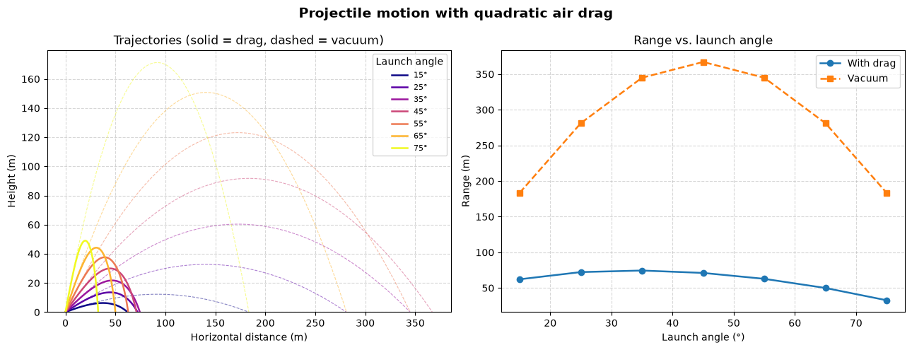
Compute projectile trajectories under gravity and quadratic air drag. Integrate the equations of motion with a fourth-order Runge-Kutta method, then compare the trajectories and ranges with the solution without drag.
[1]:
import numpy as np
import matplotlib.pyplot as plt
Physical Parameters
Use SI units throughout. The constant b combines the air density, cross-sectional area, and drag coefficient. The drag force opposes the velocity:
[2]:
g = 9.80665  # gravitational acceleration, m/s²
v0 = 60.0  # launch speed, m/s
b = 0.003  # drag constant, kg/m  (≈ baseball-sized sphere)
m = 0.145  # projectile mass, kg
RK4 Integrator
Store horizontal and vertical positions and velocities in the state vector:
Compute the speed from the velocity components:
Drag slows the horizontal motion. Gravity and drag determine the vertical acceleration:
Use a fourth-order Runge-Kutta step to advance the state. Stop the simulation when the projectile first falls below ground level after launch.
[3]:
def derivatives(state):
    """Compute velocity and acceleration under gravity and quadratic drag.

    Parameters
    ----------
    state : ndarray of shape (4,)
        Horizontal and vertical positions in meters, followed by the
        corresponding velocities in meters per second.

    Returns
    -------
    ndarray of shape (4,)
        Horizontal and vertical velocities, followed by the corresponding
        accelerations in meters per second squared.
    """
    x, y, vx, vy = state
    v = np.sqrt(vx**2 + vy**2)
    ax = -(b / m) * v * vx
    ay = -g - (b / m) * v * vy
    return np.array([vx, vy, ax, ay])
[4]:
def rk4_step(state, dt):
    """Advance the projectile state with a fourth-order Runge-Kutta step.

    Parameters
    ----------
    state : ndarray of shape (4,)
        Horizontal and vertical positions in meters, followed by the
        corresponding velocities in meters per second.
    dt : float
        Time step in seconds.

    Returns
    -------
    ndarray of shape (4,)
        Projectile state after one time step.
    """
    k1 = derivatives(state)
    k2 = derivatives(state + 0.5 * dt * k1)
    k3 = derivatives(state + 0.5 * dt * k2)
    k4 = derivatives(state + dt * k3)
    return state + (dt / 6.0) * (k1 + 2 * k2 + 2 * k3 + k4)
[5]:
def simulate(angle_deg, dt=0.01):
    """Simulate until the projectile falls below ground level after launch.

    Parameters
    ----------
    angle_deg : float
        Launch angle in degrees above the horizontal.
    dt : float, optional
        Time step in seconds. Default is 0.01.

    Returns
    -------
    xs : ndarray
        Horizontal positions in meters, including the first point below
        ground level.
    ys : ndarray
        Vertical positions in meters at the same time steps.
    """
    theta = np.radians(angle_deg)
    state = np.array([0.0, 0.0, v0 * np.cos(theta), v0 * np.sin(theta)])
    xs, ys = [state[0]], [state[1]]
    while True:
        state = rk4_step(state, dt)
        xs.append(state[0])
        ys.append(state[1])
        if state[1] < 0 and len(xs) > 2:
            break
    return np.array(xs), np.array(ys)
Compute Trajectories
Compute trajectories at seven launch angles, from 15° to 75°.
[6]:
angles = [15, 25, 35, 45, 55, 65, 75]
trajectories = {a: simulate(a) for a in angles}
[7]:
# Compute the parabolic trajectories without drag for comparison.
def simulate_vacuum(angle_deg, dt=0.01):
    """Compute the projectile trajectory without air drag.

    Parameters
    ----------
    angle_deg : float
        Launch angle in degrees above the horizontal.
    dt : float, optional
        Unused. The trajectory uses 500 equally spaced time samples.

    Returns
    -------
    xs : ndarray
        Horizontal positions in meters from launch to landing.
    ys : ndarray
        Vertical positions in meters at the same time samples.
    """
    theta = np.radians(angle_deg)
    vx0, vy0 = v0 * np.cos(theta), v0 * np.sin(theta)
    t_flight = 2 * vy0 / g
    t = np.linspace(0, t_flight, 500)
    return vx0 * t, vy0 * t - 0.5 * g * t**2
[8]:
vacuum = {a: simulate_vacuum(a) for a in angles}
Plot Trajectories and Ranges
Compare trajectories with and without drag on the left. On the right, plot the horizontal range at each launch angle.
[9]:
cmap = plt.cm.plasma
colors = [cmap(i / (len(angles) - 1)) for i in range(len(angles))]
[10]:
fig, (ax_traj, ax_range) = plt.subplots(1, 2, figsize=(13, 5))
fig.suptitle(
    "Projectile motion with quadratic air drag", fontsize=14, fontweight="bold"
)
# Use solid lines for drag and dashed lines for vacuum trajectories.
for angle, color in zip(angles, colors):
    x, y = trajectories[angle]
    xv, yv = vacuum[angle]
    ax_traj.plot(x, y, color=color, linewidth=1.8, label=f"{angle}°")
    ax_traj.plot(xv, yv, color=color, linewidth=0.8, linestyle="--", alpha=0.5)
ax_traj.set_xlabel("Horizontal distance (m)")
ax_traj.set_ylabel("Height (m)")
ax_traj.set_title("Trajectories (solid = drag, dashed = vacuum)")
ax_traj.set_ylim(bottom=0)
ax_traj.grid(True, linestyle="--", alpha=0.5)
ax_traj.legend(title="Launch angle", fontsize=8)
# Compare the range at each launch angle.
ranges_drag = [trajectories[a][0][-1] for a in angles]
ranges_vacuum = [vacuum[a][0][-1] for a in angles]
ax_range.plot(
    angles, ranges_drag, "o-", color="tab:blue", linewidth=1.8, label="With drag"
)
ax_range.plot(
    angles, ranges_vacuum, "s--", color="tab:orange", linewidth=1.8, label="Vacuum"
)
ax_range.set_xlabel("Launch angle (°)")
ax_range.set_ylabel("Range (m)")
ax_range.set_title("Range vs. launch angle")
ax_range.grid(True, linestyle="--", alpha=0.5)
ax_range.legend()
plt.tight_layout()
plt.show()
Compare Ranges
Print the launch angle with the greatest range among the seven angles tested.
[11]:
opt_drag = angles[np.argmax(ranges_drag)]
opt_vacuum = angles[np.argmax(ranges_vacuum)]
print(f"Optimal angle (drag)   : {opt_drag}°  →  range = {max(ranges_drag):.1f} m")
print(f"Optimal angle (vacuum) : {opt_vacuum}°  →  range = {max(ranges_vacuum):.1f} m")
Optimal angle (drag)   : 35°  →  range = 74.5 m
Optimal angle (vacuum) : 45°  →  range = 367.1 m