Monte Carlo Estimation of π
Estimate π by sampling points uniformly from a square that contains a unit circle. The square has side length 2, so the ratio of their areas is:
\[\frac{A_{\mathrm{circle}}}{A_{\mathrm{square}}} = \frac{\pi}{4}\]
Use the fraction of points inside the circle to estimate this ratio.
[1]:
import numpy as np
import matplotlib.pyplot as plt
Simulation Setup
Set a fixed random seed so repeated runs use the same samples.
[2]:
rng = np.random.default_rng(seed=42)
[3]:
N = 50_000 # total number of random points
Run the Simulation
Draw 50,000 points uniformly from the square:
\[(x, y) \in [-1, 1] \times [-1, 1]\]
A point lies inside the unit circle when:
\[x^2 + y^2 \leq 1\]
Count those points and compute the estimate:
\[\hat{\pi} = 4\frac{N_{\mathrm{inside}}}{N}\]
[4]:
x = rng.uniform(-1, 1, N)
y = rng.uniform(-1, 1, N)
inside = x**2 + y**2 <= 1.0
[5]:
pi_estimate = 4 * inside.sum() / N
print(
    f"π estimate after {N:,} samples: {pi_estimate:.6f}  (error: {abs(pi_estimate - np.pi):.2e})"
)
π estimate after 50,000 samples: 3.146320 (error: 4.73e-03)
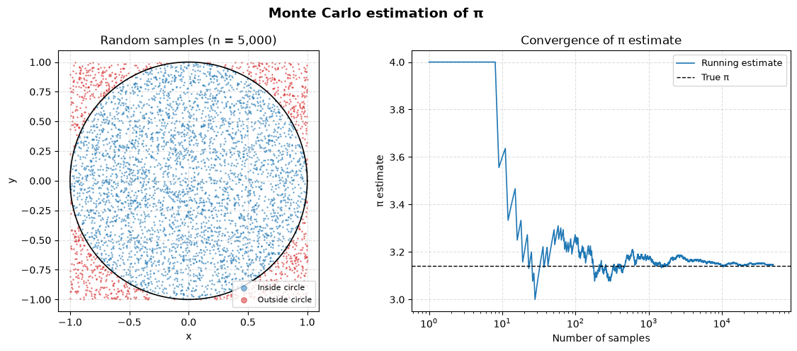
Convergence of the Estimate
Compute a running estimate after each sample. The count of points inside the circle accumulates as more points are drawn:
\[\hat{\pi}_n = 4\frac{N_{\mathrm{inside}}(n)}{n}\]
[6]:
sample_counts = np.arange(1, N + 1)
running_pi = 4 * np.cumsum(inside) / sample_counts
Plot Samples and Convergence
Show the first 5,000 points on the left, colored by whether they fall inside the circle. Plot the running estimate on the right and compare it with π.
[7]:
fig, (ax_scatter, ax_conv) = plt.subplots(1, 2, figsize=(12, 5))
fig.suptitle("Monte Carlo estimation of π", fontsize=14, fontweight="bold")
# Use the first 5,000 points to keep the scatter plot readable.
n_scatter = 5_000
ax_scatter.scatter(
    x[:n_scatter][inside[:n_scatter]],
    y[:n_scatter][inside[:n_scatter]],
    s=0.8,
    color="tab:blue",
    alpha=0.5,
    label="Inside circle",
)
ax_scatter.scatter(
    x[:n_scatter][~inside[:n_scatter]],
    y[:n_scatter][~inside[:n_scatter]],
    s=0.8,
    color="tab:red",
    alpha=0.5,
    label="Outside circle",
)
theta = np.linspace(0, 2 * np.pi, 300)
ax_scatter.plot(np.cos(theta), np.sin(theta), color="black", linewidth=1.2)
ax_scatter.set_aspect("equal")
ax_scatter.set_title(f"Random samples (n = {n_scatter:,})")
ax_scatter.set_xlabel("x")
ax_scatter.set_ylabel("y")
ax_scatter.legend(loc="lower right", markerscale=6, fontsize=8)
ax_scatter.grid(True, linestyle="--", alpha=0.4)
# Plot the running estimate against the number of samples.
ax_conv.semilogx(
    sample_counts, running_pi, color="tab:blue", linewidth=1.2, label="Running estimate"
)
ax_conv.axhline(np.pi, color="black", linewidth=1.0, linestyle="--", label="True π")
ax_conv.set_title("Convergence of π estimate")
ax_conv.set_xlabel("Number of samples")
ax_conv.set_ylabel("π estimate")
ax_conv.legend(fontsize=9)
ax_conv.grid(True, linestyle="--", alpha=0.4)
plt.tight_layout()
plt.show()
Estimate Error
Compare the final estimate with NumPy’s value of π.
[8]:
print(f"True π              : {np.pi:.6f}")
print(f"Estimated π         : {pi_estimate:.6f}")
print(f"Absolute error      : {abs(pi_estimate - np.pi):.2e}")
print(f"Relative error      : {abs(pi_estimate - np.pi) / np.pi * 100:.4f} %")
True π              : 3.141593
Estimated π         : 3.146320
Absolute error      : 4.73e-03
Relative error      : 0.1505 %